Abstract
Vineyards are expanding rapidly in California's north coast due to a booming wine market. In Sonoma County, much of this expansion is occurring on hillsides that harbor California's remaining oak woodlands. The pattern of vineyard development is influenced by physiographic, environmental, and land-use variables. Two statistical methods are used to examine which physical attributes are significantly related to vineyard development: 1) Ratios were calculated that are proportional to the probability of a particular site being planted in vineyard given that the entire landscape is developable. 2) Logistic regression was used to determine the relationship between physical variables and the probability of vineyard development. The ratio model was easier to calculate, while the logistic regression model allowed for the weighting of variables and found the most significant combination of variables. Maps of suitable areas for future vineyard development were created using both techniques. These possible patterns of vineyard expansion can then be used to explore land-use planning and ecological effects. For example, we identified areas where vineyard development could lead to oak woodland fragmentation.
Introduction
California wines have become extremely popular nationally and internationally, leading to increased demand for wine grapes. In 1996 California wine grapes were worth $2.1 billion, as compared to $647 million in 1988. This increase is due both to increased price per ton and continued establishment of approximately 100,000 acres of new vineyards throughout California in the past decade, a 30 percent increase in vineyard land. Even in lesser-known wine grape growing areas such as San Luis Obispo County, an estimated 2,000 acres of rangeland is being converted to vineyard a year.
Upland areas, historically considered marginal agricultural land, are increasingly targeted for vineyard development. In some areas, the conversion from woodlands and forestland to vineyard is extensive. For example, Santa Barbara County Planning Department reported that the amount of vineyard has doubled to 20,000 acres since 1996 leading to the loss of over 2,000 oak trees, a larger number than all rural development and subdivisions were responsible for removing in the past ten years. In Sonoma County, we have estimated that at least 1,660 acres of oak woodland were lost to vineyard development between 1990 and 1997. Sonoma County has also seen a 31.5% growth in vineyard area in that time period (4720.2 hectares), for a total of 19,706.6 ha.
In order to address the consequences of vineyard expansion we wanted to understand which of the remaining areas in Sonoma County are suitable for future vineyard development based on recent trends (see figure 1 for the location of Sonoma County). Therefore, we incorporated a map of Sonoma County’s vineyards into a Geographic Information System and then used statistical methods to identify which landscape variables are related to vineyards. We were then able to map suitable areas for vineyard development based on this information.
Having a probability surface for vineyard suitability allowed us to address several land-use issues that may impact the future landscape of Sonoma County including habitat fragmentation, a concern since most woodland is in private ownership and is not protected by the state regulations.
Methods
GIS Development
We were able to build vineyard expansion models for Sonoma County because vineyards had been mapped by a local grape growers association and digitized by Circuit Rider Productions, Inc (CRP). Two sources were used for vineyard mapping: 1990 non-orthorectified aerial photographs, and maps provided by the grape growers for the 1990 to 1997 time period. This map shows vineyards for most of Sonoma County except for the coast, including the Alexander Valley, Russian River Valley, Chalk Hill, Dry Creek Valley, Knights Valley, Los Carneros, Sonoma Mountain, and Sonoma Valley appellation areas (figure 2). The vineyard location data was provided as AutoCAD DXF files and converted to an Arc/Info GIS layer for further analysis. We labeled each vineyard polygon with a pre- or post-1990 establishment date based upon the source data.
This data was then incorporated into a geographic information system (GIS) and integrated with other GIS data that captures the physiographic and climatological factors that might affect where vineyards are established. The primary physiographic variables we analyzed were slope, aspect, elevation, and soils. These variables are also climatological, however, as they affect a vineyard's microclimate. We also analyzed precipitation levels and several variables that have not been included in previous analyses, but that might be influential on where a vineyard is established. These were distance from perennial streams for post-1990 vineyards, proximity of post-1990 vineyard to a pre-existing (pre-1990) vineyard, distance from roads for post-1990 vineyards, existing land-use, designated appellation region (also known as viticultural area), and existing vegetation. Interviews with viticulture experts confirmed that these variables could be influential.
The GIS data collected to analyze these variables came from a variety of sources. The slope and aspect layers were derived from 30-meter USGS Digital Elevation Models (DEM) that were downloaded from the California Geographical Survey website at the California State University at Northridge (http://geogdata.csun.edu/). The streams and roads layers were 1:100,000 TIGER94 files also downloaded from the CSU-Northridge web site. Proximity to existing vineyards was calculated by using a data layer of Sonoma County's vineyards described above. We used the California Department of Conservation's Farmland Mapping and Monitoring Project (FMMP) "farmland map" of Sonoma County to show land-use. In addition to showing the locations of farmland and grazing land, this layer also includes the extent of urban areas in the County. We used data from the 1996 version of the FMMP for the ratio model and the 1990 version for the logistic regression model. Mean annual precipitation was obtained from the Teale Data Center under a site license with the University of California - Berkeley. Appellation region was obtained from CRP along with the vineyard locations layer. We used: the "Wildlife Habitat Map for the Oregon-California Klamath Bioregion" created by the Klamath Bioregional Assessment Project at Humboldt State University and based on 1994 satellite imagery for the ratio model. We used a California Department of Forestry hardwood vegetation layer based on 1990 satellite imagery for the logistic regression model.
Ratio Calculations
This method was used to see if a particular land-use or land-cover type is over or under-represented in each category relative to this category's total availability in the landscape. For example, we divided the elevation GIS layer for Sonoma County into 100-meter bands from 0 to 800 meters, and one band for elevations above 800 meters where no vineyards were known to occur. Using ArcView's "tabulate areas" function, the "new vineyards" (those established after 1990) were intersected with the 9 slope categories. We also tabulated the area of each category for the entire county. From this, we could see that 58.0% of new vineyards have been established on areas of 0-100 meters, and 34.9% of the county ranges from 0 to 100 meters in elevation, a ratio of 1.66 to 1 of "use" to "availability". On the other hand, 6.5% of new vineyards were established on areas of 200 to 300 meters, but only 16.4% of the county is in this elevation band, a ratio of 0.42 to 1. To see if the difference between availability and use was statistically different, we applied 95% confidence intervals using the Bonferroni correction (Neu et al. 1974, Stoms et al. 1992). This gave allowed us to see if particular categories were statistically under- or over-represented for new vineyards. If the ratio was greater than 1, and the corrected confidence interval did not include 1 (such as 1.66 +/- 0.06), then post-1990 vineyards were over-represented in that category. If the ratio with intervals included 1 (such as 1.07 +/- 0.08), vineyards were using that category in proportion to its availability. If the ratio was less than 1 and did not include 1 in the confidence interval, then the new vineyards were under-represented in this category. If a category was over-represented, we gave it a "+1" value; if it was under-represented, we gave it a "-1" value, and if it was not statistically different, a 0 value was assigned (see Agee et al. 1989 for an example of this method). We converted each of the layers to a 30m Arc/Info grid, calculated each category to its -1, 0, or +1 value, and summed them using the GRID addition function. This yielded values ranging from -10 to +10. A value of -10 meant that a grid cell was under-represented for its category in each of the 10 analyzed layers. For example, a cell might be on a high elevation, far from a road, far from existing vineyards, and on a very steep slope. A value of +10 meant that a grid cell was over-represented for each category in all the analyzed layers. If a cell had 5 over-represented categories but 3 under-represented ones, it would receive a +2 value overall. The resulting grid of -10 to +10 values represented a vineyard suitability surface for the county. This surface was then available for us to model vineyard growth rates and calculating the impact on forest loss, along with other applications.
Logistic Regression
Logistic regression analysis is appropriate when the response variable is binary (e.g. 1 = post-1990 vineyard, 0 = not post-1990 vineyard) and when independent variables are categorical or continuous. For this project, logistic regression allowed us to calculate the probability that a given unit of land will become vineyard based on its physical characteristics and recent expansion patterns. Logistic regression analysis is different from the ratio calculations in that it takes into account the relative importance of each variable in determining vineyard suitability.
For this model, we added distance to nearest urban area and tested the importance of this spatial variable. We also replaced the 1994-dated Klamath vegetation layer with the 1990-dated California Department of Forestry "hardwood pixel" layer. The rest of the GIS layers were similar to those used in the ratio-model: pre-1990 and post-1990 vineyard locations, elevation, slope, aspect, agricultural and urban landuse from the 1990 Farmland Mapping and Monitoring Project, distance to roads, distance to existing (pre-1990 vineyards), distance to perennial streams, precipitation, and public land. All layers were converted to grids with a resolution of 1 ha (100 m x 100 m). All 1 ha grids were created using a reference grid of the same size so that grids could be easily overlaid. Each hectare represented a single observation for statistical analysis and had a corresponding value for each of the data layers.
Logistic regression analysis requires that all categorical variables be coded as binary dummy variables. For example, each of the 7 land-use categories became a new variable so that there was a ‘grazing’ variable, an ‘urban’ variable, etc. If a cell was classified as urban, its ‘urban’ value was 1. If it was classified as one of the other 6 land-uses, its ‘urban’ value was 0. In accordance with this requirement, binary dummy grids were derived from all 1 ha grids representing categorical variables. The dependent variable was also represented with a binary grid. A value of 1 indicated that the cell was a post-1990 vineyard and a value of 0 indicates that it was not.
We developed a mask of land not available to vineyard development in time for the logistic regression model. This mask consisted of public land, urban areas, areas already in vineyard, elevations greater than 800 meters, slopes greater than 50 percent (26.6 degrees) and water bodies. The cutoffs of 800 meters and 50 percent were chosen because the Sonoma County vineyard layer had no vineyards above 800 meters, and a new county ordinance prohibits development on slopes greater than 50 percent.
In order to test the ability of models to predict vineyard expansion, spatially distinct post-1990 vineyards were split into 2 sets, a model building set and a model testing set. Random sampling of these spatially distinct vineyards was stratified by appellation area and size class. Vineyards were grouped into 3 size classes: large (³ 100 ha), medium (<100 ha and ³ 10 ha), and small (<10 ha). One-half of the vineyards within each appellation-size class were randomly assigned to the build set and the other half to the test set. Stratification by appellation region ensured that vineyards in each set were well distributed throughout the county. Stratification by size ensured that vineyard size distribution was similar for each set, resulting in similar numbers of vineyard observations. The build set had a total of 2233 post-1990 vineyard observations, while the test set had a total of 2132. In order to randomly select non-vineyard observations, a 100 m grid of random values was created using the RANDOM command in GRID. From this grid, another grid was derived that contained these values only for 1990 available cells that did not become vineyard. The desired number of non-vineyard cells was selected by taking that number of cells with the largest random number assignments. All model testing was conducted using a single data set with a 1:1 ratio of non-vineyard to vineyard observations. Non-vineyard cells were selected using the random grid from above.
Site characteristics (e.g. vineyard or non-vineyard, elevation, slope, distance from urban areas, etc.) were extracted for each model building cell using the SAMPLE command in grid. The resulting ASCII file was imported into EXCEL for data manipulation and then into SAS for analysis. Each cell and its related characteristics were treated as an independent observation in statistical analyses.
Logistic regression models are generalized linear models where:
ln(probability of event/probability of no event) = ln(odds) = b0 + b1var1 + ... + bnvarn), where ln is the natural log.
For any logistic regression model, the odds of an event (or no event) given a set of conditions can be determined by calculating
odds = e^( b0 + b1var1 + ... + bnvarn)
Finally, logistic regression allows one to determine the probability of an event (or no event) in a given cell. Probability is calculated as
probability = odds/(1+odds)
Logistic regression has very few assumptions. However, an important assumption is that the ratio of successes to failures in a sample is not close to 1 or 0. It is for this reason that we sampled the vineyard and non-vineyard cells for model building in disproportion to their availability in Sonoma County, treating this as a case-control study.
The most complex logistic model included 35 explanatory variables. These variables represented elevation, slope, aspect (north, northeast, east, southeast, south, southwest, northwest, flat; west was used as baseline), vegetation (blue oak woodland, coast live oak woodland, montane hardwood, unclassified hardwood, conifer, shrub, urban, other; grass was used as baseline), land-use (primary farmland, unique farmland, farmland of local importance, farmland of state importance, other; grazing land was used as baseline), distance to nearest perennial stream, distance to nearest road, distance to nearest pre-1990 vineyard, and distance to nearest 1990 urban area. Eight of the variables were interaction terms: aspect*slope (north*slope, northeast*slope, east*slope, southeast*slope, south*slope, southwest*slope, northwest*slope; west*slope used as baseline) and elevation*slope. Aspect*slope takes into account changes in the effect of aspect on vineyard suitability as slope changes, and elevation*slope takes into account changes in the effect of elevation on vineyard suitability as slope changes.
Using the most complex model as a starting point, categorical variables were combined using backward stepwise regression and information theory in the following manner. Each logistic regression model received a Akaike Information Criteria (AIC) value based on its ability to describe the input data (see Burnham and Anderson, 1998). The lower the AIC value, the closer to "truth" the model is believed to be (Akaike, 1973). In performing a backward stepwise regression, we repeatedly selected the model with one less variable that had the lowest AIC value. For example, since we started with a model with 35 variables, the next step was to build multiple models with 34 variables. In doing so, we chose to remove a variable (making it part of the baseline) or combine 2 variables into a single variable (e.g. blue oak woodland and coast live oak woodland may be combined into a single variable that represents oak woodland). The 34-variable model that had the lowest AIC value was chosen as the best model with 34 variables. Multiple models with 33 variables were then built using the best 34-variable model as a reference. The best 33-variable model was selected using AIC values. This process continued until no model with a lower AIC value could be found. Out of all models built, the model with the lowest AIC value was chosen as the final model. Continuous variables were not removed at any point in this process.
In order to determine the classification accuracy of the final model, the equation from the model was used to calculate the probability value for each cell in the model testing sample. The 2132 (the actual number of post-1990 vineyard observations) cells with the highest probabilities were classified as vineyard, and the 2156 (the actual number of non-vineyard observations) cells with the lowest probabilities were classified as non-vineyard. For each cell, the classification was compared with whether or not the cell actually became vineyard. Classification accuracy was calculated as
(number of cells classified correctly/total number of cells classified) * 100%
A probability surface was created for the entire county by applying the equation from the final model to each cell. This was done using map algebra in GRID.
Consequences for Habitat Fragmentation
In order to identify where vineyard expansion may lead to forest fragmentation in the future, we identified changes in habitat connectivity if vineyards were developed in areas with a suitability level of p>0.5 using the logistic regression model. We calculated core areas of oak woodland using the "core.aml" program from Shawn Saving and Greg Greenwood of the California Department of Forestry (CDF). This program uses an GRID layer of a county's vegetation to calculate the core areas of oak woodland. A core area was defined as at least 100 hectares in size, at least 50 meters (two 25 meter pixels) away from urban areas, and within 25 meters (1 pixel) of other oak woodland pixels. These land-cover classes were available in the "CDF hardwood pixel" vegetation layer based on 1990 Landsat Thematic Mapper imagery that we had previously obtained from CDF. The core variables are user-definable, but we used those suggested by Shawn Saving.
Using the core program, we calculated the core oak woodland at the "current" time period, which reflected the 1990 date of the source imagery. We then took our maximum development scenario from the logistic regression model and converted all of the greater than 0.5 development probability areas that were in oak woodland to the "grass" class, which is what most vineyards had been classified as by the CDF. We ran the core program with this reclassified layer and obtained the number and size of the core areas under a possible vineyard expansion scenario and noted areas where development would fragment large forest patches and make smaller forest patches disappear.
Results
Statistical Methods
The results from our statistical analysis demonstrate which variables are correlated with where vineyards are on the landscape and allowed us to map suitable areas for vineyard planting in Sonoma County based on past trends of agricultural development
The ratios and Bonferroni-corrected confidence intervals are summarized in table 1 (see the appendix). Adding together the 10 variables into a single GIS layer produced the vineyard suitability layer in figure 3. For the ratio model, vineyards were over-represented in (or "associated with") elevations < 100 m, slopes < 10 degrees, precipitation < 35 inches per year, the Los Carneros and Alexander Valley appellation areas, areas not immediately adjacent to perennial streams (mostly in the 600-2200 m range), near existing vineyards (<1200 m), near roads (<200m), existing farmland, northeast and east aspects, and the following vegetation classes: dead grass/forb, rock/gravel, soil, and unclassified areas.
The 17-variable logistic regression model we used was:
Log odds = 1.1795 - 0.00210*elevation - 0.0383*slope + 0.000088*(elevation*slope) + 0.3938*(east + southeast + south + north) + 0.6663*(northeast + northwest) - 0.3914*(flat) - 0.0170*(southeast*slope + northwest*slope) + 0.6065*(local farmland + prime farmland) + 1.1862*(unique farmland + statewide farmland) - 0.7926*(other use) - 1.1239*(montane hardwood + potential hardwood + coast live oak woodland) - 0.4428*(conifer) - 0.9140*(urban cdf)+ 0.000281*(distance to 1990 urban areas) + 0.00021*(distance to perennial streams) - 0.00082*(distance to pre-1990 vineyards) - 0.00008*(distance to roads)
The probability surface resulting from the selected logistic regression model is presented in figure 4. Using the test half of the new vineyards data set, we calculated the accuracy of the logistic regression model to be 77%.
For the logistic regression model, the following variables decrease the probability of a cell becoming vineyard: increasing elevation, increasing slope, and increasing distance from existing vineyards. The following variables increased the probability of a cell becoming vineyard: increasing distance to nearest perennial stream, increasing distance from urban areas, if the area was in grass, shrub, blue oak woodland, or "other" vegetation in the 1990 CDF layer; if farmland was already present in 1990, if the slopes were facing northwest or northeast. Blue oak woodland, grass, shrub, or "other vegetation" were the most likely vegetation types to be developed into vineyard, followed by conifer, and then urban. Montane hardwood, unclassified hardwood, and coast live oak woodland were the least likely to be developed. Unique farmland and farmland of state importance were the most likely land use types to be developed, followed by prime farmland and farmland of local importance, and then grazing land. "Other land" was the least likely land use type to be developed. Northeast and northwest facing slopes had the highest probability of being developed. East, southeast, south, and north facing slopes had the next highest probability of being developed, followed by northwest, southwest, and west facing slopes. Flat slopes (defined as slopes with no discernible aspect in the digital elevation model) were the least likely to be developed. Vineyards were less likely to be developed on steep slopes on northwest and southeast facing slopes than on other aspect categories. Finally, increasing elevation meant that vineyards were more likely to be established on steeper slopes.
Consequences for Habitat Fragmentation
Using the 1990 CDF vegetation layer, we calculated that there were 72 core areas of oak woodland, totaling 88,279 ha, of which 7 were larger than 4,000 ha and 36 were between 100 ha (our mininum size for core areas) and 200 ha. We chose a greater than 0.5 probablility level from the logistic regression model as our "maximum vineyard development scenario" for the fragmentation analysis. This level included a large amount of vineyard (93,587 ha, or 23% of Sonoma County's area), and signified a "better than even" chance for development. After changing all areas in the logistic regression model with a probability greater than 0.5 into vineyard, we calculated that there were 76 core oak woodland areas, totaling 75,814 ha (a decline of 14.1% in area), with only 4 being greater than 4,000 ha and 32 in the 100 to 200 ha size. The increased count of core areas was due to the larger core areas being split into several smaller ones. An example of the potential fragmentation of oak woodlands is shown for the Jimtown area in the northeast part of Sonoma County in figure 5. Four areas of change in oak woodland connectivity or extent are shown with labels A, B, C, and D. Labels A and D show new core fragments that had previously been connected to a larger core area of oak woodland, and B and C are former core areas that disappear because of potential vineyard development.
Discussion
This research provides a comparison of two methods for examining suitable areas for vineyard development and demonstrates the utility of modeling probability surfaces for land-use change that is resulting in deforestation.
Digital Data
As we developed the ratio model and then the logistic regression model, we refined some our input data choices. It became clear that it was unacceptable to use a vegetation map derived from imagery taken in 1994 in an analysis of vineyard expansion between 1990 and 1997. The vegetation variable of interest is vegetation prior to development, yet this value would be undeterminable for about half of the post-1990 vineyard cells. Hence, we switched to the CDF hardwood map to determine 1990 vegetation type. For similar reasons, we used the 1990 FMMP landuse layer in the regression model instead of the 1996 version we used in the ratio model.
For the ratio model, we used whatever the native grain of layer was, from the 30 m Klamath vegetation layer to the multi-sized polygons of the farmland layer. For the logistic regression model, all the data layers were transformed to 1 ha cells before being input into the model. The following reasoning was used to determine 1 ha as the unit of analysis. Several of the available GIS layers have a 30 m (900 m2) cell size. Thus, 30 m2 could have been chosen as the unit of analysis in order to retain as much information from the original GIS layers as possible. However, the amount of data that would be created by using a 30 m cell size would be too large for analysis. Instead of 410,694 observations (already a large amount) for Sonoma Co. if 1 ha cells are used, there would be 4,563,267 observations if 30 m cells are used. Furthermore, because vineyard locations were mapped using non-orthorectified aerial photos, spatial error in vineyard location is sometimes as high as 150 m. Using a 30 m cell size would represent a level of accuracy that simply does not exist in the data. On the other hand, using a cell size much larger than 1 ha would be problematic because much of the on-the-ground information that growers use in making development decisions would be lost. The average size of spatially distinct post-1990 vineyards in Sonoma Co. was 9.7 ha, and the vast majority (400 out of 558) were larger than 1 ha. Thus, treating the landscape as 1 ha plots reflects the scale at which a developer might look at the land.
We used the mean annual precipitation layer in the ratio model but not in the regression model. The logistic regression model is sensitive to having a minimum number of observations in each category of a categorical variable. This was not the case for precipitation, as some of the wide bands of the 1:1,000,000 scale layer had few or no vineyards in them.
Soils data, often considered one of the most important variables that affects vineyards (Seguin, 1986), was not available in a GIS format for Sonoma County. We undertook the digitizing of the 1972 Soil Conservation Service soil survey for the county. Because this work is still in progress, we were not able to incorporate it in our vineyard expansion models at the time of writing this paper. We anticipate that future versions will include this variable, including additional soils-based variables such as clay content, cation exchange capacity, organic matter content, soil depth, mineral content, erosion potential, Storie index, water-holding capacity, and others (Watkins, 1997).
Statistical Methods
The utility of the ratio method is in the fact that the ratios are relatively easy to calculate and the results are easier for the public and policy makers to understand. Also, the ratio model gives "degrees" of unsuitability with the -10 to -1 values and suitability with the 1 to 10 values, while regression model gives the probability of being suitable. If we have mapped an area as unsuitable for vineyards, we can still calculate relative suitability if we discover that such an area is likely to be developed anyway.
The logistic regression methods provided us with a probability surface that allows us to identify which combination of variables were important for determining a suitable vineyard site. I In addition, we took correlation between layers into account through the variable weights in the regression equation. The ratio model treated all variables as equally significant, and did not address correlation. This is because ratio models have traditionally only been used for a single variable, such as land cover (Neu et al. 1974, McClean et al. 1998).
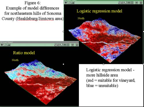
While the general trends of the models are similar (see figures 3 and 4), there are some differences. The ratio model predicts more land as suitable in the southern tip of the county and in some coastal areas, while the logistic regression model predicts more suitable land in the northeast county hillsides. An example of this can be seen in the 3-D scenes of the Jimtown/Healsdburg area from the northeast part of the county (figure 6). The lack of suitability in the coasts and the greater suitability in the hillsides is most likely due to the heavy weighting of the "distance to existing vineyards" variable in the logistic regression model. As no vineyards were mapped on the coast (because the mapping project excluded this area), these areas were far from existing vineyards, so the logistic regression model predicted these areas as unsuitable.
Another difference is that the ratio model had a relatively normal data distribution, while the logistic regression model had a majority of values in the most unsuitable areas (see the histogram in figure 7). We are evaluating this difference to see if the skew towards unsuitable areas in the regression model reflects a real-world trend or is an artifact of the modeling process.
Consequences for Habitat Fragmentation
The methods used allowed us to do more than identify areas of potential habitat loss. By comparing the forest patches before and after conversion of areas suitable for vineyard development we are able to identify priority sites that if protected could prevent fragmenting the largest remaining forested areas in Sonoma County. We are currently working with the Sonoma County Agricultural Preservation and Open Space District on updating their conservation easement acquisition plan so that these areas at high risk from forest loss and fragmentation could be protected from vineyard development. As our work so far shows both forest loss and fragmentation from vineyard expansion, we have the opportunity to inform government agencies and environmental groups concerned with environmental protection.
Future improvements and applications
We are working on several improvements in our modeling efforts. We will be addressing spatial autocorrelation within layers. We will also be making our models more "real world" as they currently reflect potential vineyard suitability and not necessarily the likelihood of development. In addition to the soil variables, we will be trying to include water availability, land pricing, land availability, yield, profit, and changes in the economy, along with other variables.
We are also working on additional applications of our models. We plan on evaluating the effects of new land use policies, such as the new ordinance that restricts vineyard developments on steep slopes. We are asking spatial questions such as "what percentage of new vineyard developments are likely to go into the different restrictions classes?" We are investigating the modeling of changes in water use as the area and number of vineyards increase. We also are looking at the interaction of expanding vineyard area with soil erosion, and studying possible effects such as changes in salmon habitat through increased sedimentation.
Acknowledgments
We would like to thank the Sonoma County Grape Growers Association for sharing their vineyard layer with us, and Circuit Rider Productions for creating the layer. Thanks also to Tim Pudoff of the Sonoma County Information Systems Department for sharing his Sonoma County GIS layers, some of which appear in the maps in this paper. Thanks to Shawn Saving and Greg Greenwood for their "core.aml." Finally, thanks to all the other cooperators in this project whom we have not named here.
Appendix
| Table 1: Summary of ratios and Bonferroni-corrected confidence intervals |
| Note: There are some differences in totals for entire county and new vineyard totals |
| for each variable due to small errors introduced in the layer intersection and summation process. |
| The area totals are all within 1% of each other. |
| Elevation variable | |||||||
| Category | Entire County Hectares | % of total | New vineyards Ha | % of total | Ratio | Confidence interval (+/-) | Value for model |
|
0-100meters |
143215.9 |
34.9% |
2733.6 |
58.0% |
1.66 |
0.06 |
+1 |
|
100-200 |
86724.3 |
21.1% |
1064.8 |
22.6% |
1.07 |
0.08 |
0 |
|
200-300 |
67410.1 |
16.4% |
324.4 |
6.9% |
0.42 |
0.06 |
-1 |
|
300-400 |
47574.2 |
11.6% |
305.0 |
6.5% |
0.56 |
0.09 |
-1 |
|
400-500 |
28995.6 |
7.1% |
177.6 |
3.8% |
0.53 |
0.11 |
-1 |
|
500-600 |
16788.0 |
4.1% |
85.8 |
1.8% |
0.45 |
0.13 |
-1 |
|
600-700 |
9585.7 |
2.3% |
23.8 |
0.5% |
0.22 |
0.12 |
-1 |
|
700-800 |
4637.3 |
1.1% |
0.0 |
0.0% |
0.00 |
0.00 |
-1 |
|
>800m |
5864.0 |
1.4% |
0.0 |
0.0% |
0.00 |
0.00 |
-1 |
|
Total |
410795.1 |
0.0% |
4715.0 |
0.0% |
0.00 |
0.00 |
-1 |
| Slope variable | |||||||
| Category | Entire County Ha | % of total (Po) | New vineyards ha | % of total | Ratio | Confidence interval | Value for model |
| 0-5 degrees |
115027.2 |
28.0% |
2469.3 |
52.4% |
1.87 |
0.08 |
+1 |
| 5-10 |
64526.7 |
15.7% |
1046.1 |
22.2% |
1.41 |
0.11 |
+1 |
| 10-15 |
63767.4 |
15.5% |
701.5 |
14.9% |
0.96 |
0.10 |
0 |
| 15-20 |
59435.1 |
14.5% |
321.1 |
6.8% |
0.47 |
0.07 |
-1 |
| 20-25 |
50299.6 |
12.2% |
119.3 |
2.5% |
0.21 |
0.05 |
-1 |
| 25-30 |
34008.9 |
8.3% |
43.0 |
0.9% |
0.11 |
0.05 |
-1 |
| 30-35 |
17268.1 |
4.2% |
11.3 |
0.2% |
0.06 |
0.05 |
-1 |
| 35-40 |
5363.4 |
1.3% |
2.6 |
0.1% |
0.04 |
0.08 |
-1 |
| 40-45 |
939.0 |
0.2% |
0.0 |
0.0% |
0.00 |
0.00 |
-1 |
| 45-50 |
124.6 |
0.0% |
0.0 |
0.0% |
0.00 |
0.00 |
-1 |
| 50-55 |
14.8 |
0.0% |
0.0 |
0.0% |
0.00 |
0.00 |
-1 |
| 55-60 |
4.0 |
0.0% |
0.0 |
0.0% |
0.00 |
0.00 |
-1 |
| 60-65 |
1.1 |
0.0% |
0.0 |
0.0% |
0.00 |
0.00 |
-1 |
| 65-70 |
0.4 |
0.0% |
0.0 |
0.0% |
0.00 |
0.00 |
-1 |
| Total |
410780.5 |
4714.2 |
|||||
| Appellation area variable | |||||||
| Category | Entire County Ha | % of total | New vineyards ha | % of total | Ratio | Confidence interval | Value for model |
| Chalk Hill |
9879.0 |
2.4% |
46.7 |
1.0% |
0.412 |
0.166 |
-1 |
| Alexander Valley |
30223.0 |
7.4% |
1136.6 |
24.1% |
3.273 |
0.235 |
+1 |
| Dry Creek Valley |
31733.2 |
7.7% |
363.6 |
7.7% |
0.997 |
0.139 |
0 |
| Knights Valley |
14868.2 |
3.6% |
435.1 |
9.2% |
2.547 |
0.323 |
+1 |
| Russian River Valley |
50448.6 |
12.3% |
895.5 |
19.0% |
1.545 |
0.129 |
+1 |
| Sonoma Mountain |
2346.0 |
0.6% |
23.5 |
0.5% |
0.871 |
0.497 |
0 |
| Sonoma Valley |
46910.4 |
11.4% |
1544.7 |
32.7% |
2.866 |
0.166 |
+1 |
| Los Carneros |
9021.2 |
2.2% |
1009.2 |
21.4% |
9.737 |
0.754 |
+1 |
| Outside App. Area in GIS cover |
238750.3 |
58.1% |
355.3 |
7.5% |
0.130 |
0.018 |
-1 |
| Total |
410843.0 |
4720.2 |
|||||
| (Note: some appellation areas overlap) | |||||||
| Precipitation variable (mean annual) | |||||||
| Category | Entire County Ha | % of total | New vineyards ha | % of total | Ratio | Confidence interval | Value for model |
| 18" |
1892.3 |
0.5% |
77.1 |
1.6% |
3.54 |
1.12 |
+1 |
| 22.5" |
27287.2 |
6.6% |
900.9 |
19.1% |
2.87 |
0.24 |
+1 |
| 27.5" |
40696.0 |
9.9% |
227.0 |
4.8% |
0.48 |
0.09 |
-1 |
| 30" |
7.0 |
0.0% |
0.0 |
0.0% |
0.00 |
0.00 |
-1 |
| 35" |
116547.4 |
28.4% |
2182.3 |
46.2% |
1.63 |
0.07 |
+1 |
| 45" |
95087.9 |
23.2% |
1136.6 |
24.1% |
1.04 |
0.08 |
0 |
| 55" |
59488.6 |
14.5% |
182.3 |
3.9% |
0.27 |
0.05 |
-1 |
| 65" |
57173.4 |
13.9% |
14.1 |
0.3% |
0.02 |
0.02 |
-1 |
| 75" |
11228.9 |
2.7% |
0.0 |
0.0% |
0.00 |
0.00 |
-1 |
| 85" |
1035.8 |
0.3% |
0.0 |
0.0% |
0.00 |
0.00 |
-1 |
| Total |
410444.5 |
4720.2 |
|||||
| Vegetation variable (Klamath bioregion) | |||||||
| Category | Entire County Ha | % of total | New vineyards ha | % of total | Ratio | Confidence interval | Value for model |
| Clouds |
5620.4 |
1.4% |
0.0 |
0.0% |
0.00 |
0.00 |
-1 |
| Dead Grass/Forb |
96150.7 |
23.4% |
1929.2 |
40.8% |
1.75 |
0.09 |
+1 |
| Deadstick Shrub |
16637.9 |
4.0% |
151.1 |
3.2% |
0.79 |
0.19 |
-1 |
| Green Grass/Forb |
33259.1 |
8.1% |
416.2 |
8.8% |
1.09 |
0.15 |
0 |
| Greenleaf Shrub |
10958.8 |
2.7% |
50.9 |
1.1% |
0.40 |
0.17 |
-1 |
| Mixed Conifer |
40220.0 |
9.8% |
109.1 |
2.3% |
0.24 |
0.07 |
-1 |
| Mixed Conifer-Hardwood |
17772.8 |
4.3% |
43.4 |
0.9% |
0.21 |
0.09 |
-1 |
| Mixed Hardwood |
33604.9 |
8.2% |
216.2 |
4.6% |
0.56 |
0.11 |
-1 |
| Mixed Hardwood-Conifer |
70057.4 |
17.1% |
157.3 |
3.3% |
0.20 |
0.05 |
-1 |
| Mixed Oak Woodland |
21308.0 |
5.2% |
130.1 |
2.8% |
0.53 |
0.14 |
-1 |
| Mixed Pine |
4553.7 |
1.1% |
20.9 |
0.4% |
0.40 |
0.26 |
-1 |
| Rock/Gravel/pavement |
19461.7 |
4.7% |
271.2 |
5.7% |
1.21 |
0.21 |
+1 |
| Soil |
21561.4 |
5.2% |
565.5 |
12.0% |
2.28 |
0.27 |
+1 |
| Unclassified |
17056.7 |
4.2% |
658.8 |
13.9% |
3.36 |
0.36 |
+1 |
| Water |
2521.5 |
0.6% |
3.4 |
0.1% |
0.12 |
0.19 |
-1 |
| Wet Meadow/Marsh |
104.5 |
0.0% |
0.2 |
0.0% |
0.15 |
1.04 |
0 |
| Total |
410849.6 |
4723.3 |
|||||
| Distance to nearest perennial stream variable | |||||||
| Category | Entire County ha | % of total | New vineyards ha | % of total | Ratio | Confidence interval | Value for model |
| 0-200m |
84152.9 |
20.5% |
668.6 |
14.2% |
0.69 |
0.05 |
-1 |
| 200-400 |
70860.1 |
17.2% |
770.4 |
16.3% |
0.95 |
0.06 |
-1 |
| 400-600 |
59573.1 |
14.5% |
723.3 |
15.3% |
1.06 |
0.07 |
0 |
| 600-800 |
48386.7 |
11.8% |
624.0 |
13.2% |
1.12 |
0.08 |
+1 |
| 800-1000 |
37406.6 |
9.1% |
559.8 |
11.9% |
1.30 |
0.10 |
+1 |
| 1000-1200 |
27822.5 |
6.8% |
362.7 |
7.7% |
1.13 |
0.11 |
+1 |
| 1200-1400 |
19894.0 |
4.8% |
258.4 |
5.5% |
1.13 |
0.13 |
0 |
| 1400-1600 |
13965.9 |
3.4% |
189.2 |
4.0% |
1.18 |
0.16 |
+1 |
| 1600-1800 |
10067.8 |
2.5% |
128.1 |
2.7% |
1.11 |
0.19 |
0 |
| 1800-2000 |
7552.9 |
1.8% |
115.0 |
2.4% |
1.33 |
0.24 |
+1 |
| 2000-2200 |
5907.2 |
1.4% |
134.0 |
2.8% |
1.97 |
0.33 |
+1 |
| 2200-2400 |
4709.1 |
1.1% |
66.7 |
1.4% |
1.23 |
0.29 |
0 |
| 2400-2600 |
3824.1 |
0.9% |
23.7 |
0.5% |
0.54 |
0.22 |
-1 |
| 2600-2800 |
3021.3 |
0.7% |
19.4 |
0.4% |
0.56 |
0.25 |
-1 |
| 2800-3000 |
2404.8 |
0.6% |
9.9 |
0.2% |
0.36 |
0.22 |
-1 |
| 3000-3200 |
1945.9 |
0.5% |
11.1 |
0.2% |
0.50 |
0.29 |
-1 |
| 3200-3400 |
1596.1 |
0.4% |
6.1 |
0.1% |
0.33 |
0.26 |
-1 |
| 3400-3600 |
1383.4 |
0.3% |
6.1 |
0.1% |
0.38 |
0.30 |
-1 |
| 3600-3800 |
1193.8 |
0.3% |
18.3 |
0.4% |
1.34 |
0.61 |
0 |
| 3800-4000 |
999.9 |
0.2% |
18.8 |
0.4% |
1.63 |
0.74 |
0 |
| 4000-4200 |
801.9 |
0.2% |
7.7 |
0.2% |
0.83 |
0.59 |
0 |
| >4200m |
3373.0 |
0.8% |
0.0 |
0.0% |
0.00 |
0.00 |
-1 |
| Total |
410842.8 |
4721.1 |
|||||
| Distance to existing vineyard variable | |||||||
| Category | Entire County ha | % of total | New vineyards ha | % of total | Ratio | Confidence interval | Value for model |
| 0-200m |
40205.9 |
9.8% |
1266.8 |
26.8% |
2.74 |
0.13 |
+1 |
| 200-400 |
18907.8 |
4.6% |
1078.8 |
22.8% |
4.96 |
0.26 |
+1 |
| 400-600 |
16203.7 |
3.9% |
688.8 |
14.6% |
3.70 |
0.26 |
+1 |
| 600-800 |
14489.3 |
3.5% |
435.8 |
9.2% |
2.62 |
0.23 |
+1 |
| 800-1000 |
12509.0 |
3.0% |
242.6 |
5.1% |
1.69 |
0.21 |
+1 |
| 1000-1200 |
10647.0 |
2.6% |
150.4 |
3.2% |
1.23 |
0.19 |
+1 |
| 1200-1400 |
9357.0 |
2.3% |
108.4 |
2.3% |
1.01 |
0.19 |
0 |
| 1400-1600 |
8637.0 |
2.1% |
111.7 |
2.4% |
1.13 |
0.21 |
0 |
| 1600-1800 |
8092.1 |
2.0% |
87.9 |
1.9% |
0.95 |
0.20 |
0 |
| 1800-2000 |
7716.0 |
1.9% |
80.3 |
1.7% |
0.91 |
0.20 |
0 |
| 2000-2200 |
7509.5 |
1.8% |
56.3 |
1.2% |
0.65 |
0.17 |
-1 |
| 2200-2400 |
7316.6 |
1.8% |
63.5 |
1.3% |
0.76 |
0.18 |
-1 |
| 2400-2600 |
6872.5 |
1.7% |
48.0 |
1.0% |
0.61 |
0.17 |
-1 |
| 2600-2800 |
6410.5 |
1.6% |
46.9 |
1.0% |
0.64 |
0.18 |
-1 |
| 2800-3000 |
6130.6 |
1.5% |
32.3 |
0.7% |
0.46 |
0.16 |
-1 |
| 3000-3200 |
5882.9 |
1.4% |
22.5 |
0.5% |
0.33 |
0.14 |
-1 |
| 3200-3400 |
5704.5 |
1.4% |
21.2 |
0.4% |
0.32 |
0.14 |
-1 |
| 3400-3600 |
5462.0 |
1.3% |
13.8 |
0.3% |
0.22 |
0.12 |
-1 |
| 3600-3800 |
5358.6 |
1.3% |
6.2 |
0.1% |
0.10 |
0.08 |
-1 |
| 3800-4000 |
5187.1 |
1.3% |
4.1 |
0.1% |
0.07 |
0.07 |
-1 |
| 4000-4200 |
4996.5 |
1.2% |
2.3 |
0.0% |
0.04 |
0.05 |
-1 |
| >4200m |
197248.4 |
48.0% |
157.6 |
3.3% |
0.07 |
0.01 |
-1 |
| Total |
410844.3 |
4721.1 |
|||||
| Distance to nearest road variable | |||||||
| Category | Entire County ha | % of total | New vineyards ha | % of total | Ratio | Confidence interval | Value for model |
| 0-200m |
190345.9 |
46.3% |
2417.5 |
51.2% |
1.11 |
0.04 |
+1 |
| 200-400 |
89662.8 |
21.8% |
1272.5 |
27.0% |
1.24 |
0.08 |
+1 |
| 400-600 |
52709.9 |
12.8% |
564.1 |
12.0% |
0.93 |
0.10 |
0 |
| 600-800 |
31417.0 |
7.6% |
289.3 |
6.1% |
0.80 |
0.13 |
-1 |
| 800-1000 |
18786.0 |
4.6% |
103.5 |
2.2% |
0.48 |
0.13 |
-1 |
| 1000-1200 |
11185.8 |
2.7% |
45.3 |
1.0% |
0.35 |
0.15 |
-1 |
| 1200-1400 |
6665.3 |
1.6% |
19.1 |
0.4% |
0.25 |
0.16 |
-1 |
| 1400-1600 |
3994.8 |
1.0% |
7.0 |
0.1% |
0.15 |
0.16 |
-1 |
| 1600-1800 |
2460.6 |
0.6% |
1.4 |
0.0% |
0.05 |
0.12 |
-1 |
| 1800-2000 |
1621.6 |
0.4% |
0.0 |
0.0% |
0.00 |
0.00 |
-1 |
| >2000m |
1992.7 |
0.5% |
0.0 |
0.0% |
0.00 |
0.00 |
-1 |
| Total |
410842.4 |
4719.7 |
|||||
| Existing land-use (FMMP 1996) variable | |||||||
| Category | Entire County ha | % of total | New vineyards ha | % of total | Ratio | Confidence interval | Value for model |
| Prime farmland |
13856.6 |
3.3% |
621.7 |
13.2% |
3.95 |
0.40 |
+1 |
| Farmland of statewide importance |
6342.2 |
1.5% |
243.0 |
5.1% |
3.37 |
0.58 |
+1 |
| Unique farmland |
8960.9 |
2.2% |
517.1 |
11.0% |
5.07 |
0.58 |
+1 |
| Farmland of local importance |
39134.3 |
9.4% |
983.3 |
20.8% |
2.21 |
0.17 |
+1 |
| Grazing land |
178510.9 |
43.0% |
1754.7 |
37.2% |
0.86 |
0.04 |
-1 |
| Urban & built-up land |
25919.7 |
6.2% |
70.9 |
1.5% |
0.24 |
0.08 |
-1 |
| Other land |
135093.3 |
32.6% |
528.1 |
11.2% |
0.34 |
0.04 |
-1 |
| Water |
7088.0 |
1.7% |
0.0 |
0.0% |
0.00 |
0.00 |
-1 |
| Total |
414905.9 |
4718.7 |
|||||
| Aspect variable | |||||||
| Category | Entire County ha | % of total | New vineyards ha | % of total | Ratio | Confidence interval | Value for model |
| Flat |
21451.5 |
5.22% |
265.0 |
5.62% |
1.076 |
0.178 |
0 |
| North |
44227.8 |
10.77% |
491.9 |
10.43% |
0.969 |
0.115 |
0 |
| NE |
48049.7 |
11.70% |
703.9 |
14.92% |
1.276 |
0.123 |
+1 |
| East |
42701.1 |
10.39% |
558.1 |
11.83% |
1.138 |
0.125 |
+1 |
| SE |
41899.8 |
10.20% |
487.3 |
10.33% |
1.013 |
0.120 |
-1 |
| South |
56665.6 |
13.79% |
606.1 |
12.85% |
0.932 |
0.098 |
-1 |
| SW |
67257.6 |
16.37% |
696.5 |
14.77% |
0.902 |
0.087 |
-1 |
| West |
50190.3 |
12.22% |
501.8 |
10.64% |
0.871 |
0.102 |
-1 |
| NW |
38351.7 |
9.34% |
406.0 |
8.61% |
0.922 |
0.121 |
0 |
| Total |
410795.1 |
4716.6 |
|||||
References
Burnham, K.P., and D.R. Anderson. 1998. Model Selection and Inference: a Practical Information - Theoretic Approach. New York, New York: Springer-Verlag New York, Inc. 353 pp.
McClean, S. A., M. A. Rumble, R. M. King, and W. L. Baker. 1998. Evaluation of resource selection methods with different definitions of availability. Journal of Wildlife Management 62(2): 793-801.
Neu, C. W., C. R. Byers, and J. M. Peek. 1974. A technique for analysis of utilization-availability data. Journal of Wildlife Management 38(3): 541-545.
Seguin, G. 1986. 'Terroirs' and pedology of wine growing. Experientia 42: 861-873.
Stoms, D. M., F. W. Davis, and C. B. Cogan. 1992. Sensitivity of wildlife habitat models to uncertainties in GIS data. Photogrammetric Engineering and Remote Sensing 58(6): 843-850.
Watkins, R. L. 1997. Vineyard site suitability in eastern California. GeoJournal 43(3): 229-239.
Author Information
Colin
Brooks
GIS Analyst
University of California - Berkeley
Integrated
Hardwood Range Management Program
Hopland Research and Extension
Center
4070 University Road
Hopland, CA 95449
Phone:
707-744-1270
Fax: 707-744-1040
E-mail:
cbrooks@nature.berkeley.edu
Emily Heaton
Graduate
student
University of California - Berkeley
1446 Loma Vista
Street
Pasadena, CA 91104
Phone: 626-798-5503
E-mail:
eheaton@nature.berkeley.edu
David Newburn
Graduate
student
University of California - Berkeley
5909 Keith Ave.
Oakland, CA
94618
Phone: 510-601-9473
E-mail:
dnewburn@nature.berkeley.edu
Adina M. Merenlender
Same contact
information as Colin Brooks
E-mail: adina@nature.berkeley.edu